|
Motion Blurred Images Generation Here we briefly illustrate the algorithms used to generate motion-blur trajectories and PSFs that have been implemented in the provided Matlab functions. Generation of Random-Motion Trajectories The createTrajectory.m function generates a variety of random motion trajectories in continuous domain as in [Boracchi and Foi 2012]. Each trajectory is represented by a complex-valued vector corresponding to the discrete positions of a particle following a 2-D random motion in continuous domain. The particle is initially characterized by a velocity vector which, at each iteration, is affected by a Gaussian perturbation and by a deterministic inertial component, directed toward the previous particle position. In addition, with a small probability, an impulsive (abrupt) perturbation aiming at inverting the particle velocity may arises, mimicking a sudden movement that occurs when the user presses the camera button or tries to compensate the camera shake. At each step, the velocity is normalized to guarantee that trajectories corresponding to equal exposures have the same length. Each perturbation (Gaussian, inertial, and impulsive) is ruled by its own parameter. Rectilinear Blur as in [Boracchi and Foi 2011] can be obtained by setting the anxiety parameter to 0 (when no impulsive changes occurs). PSF Generation
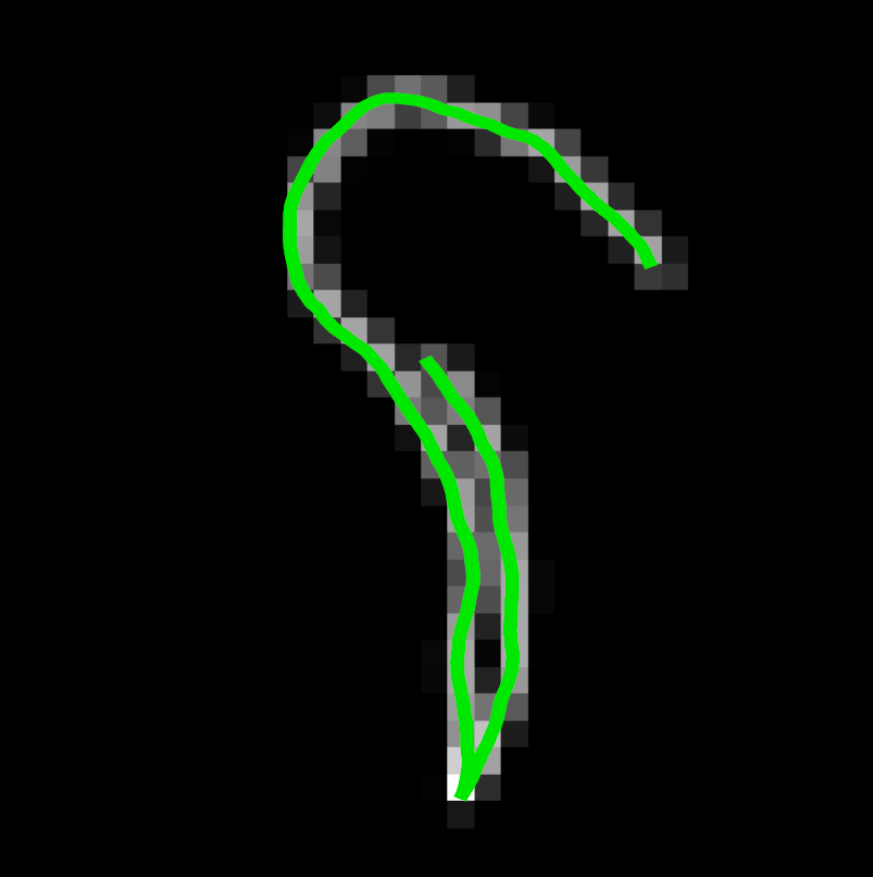
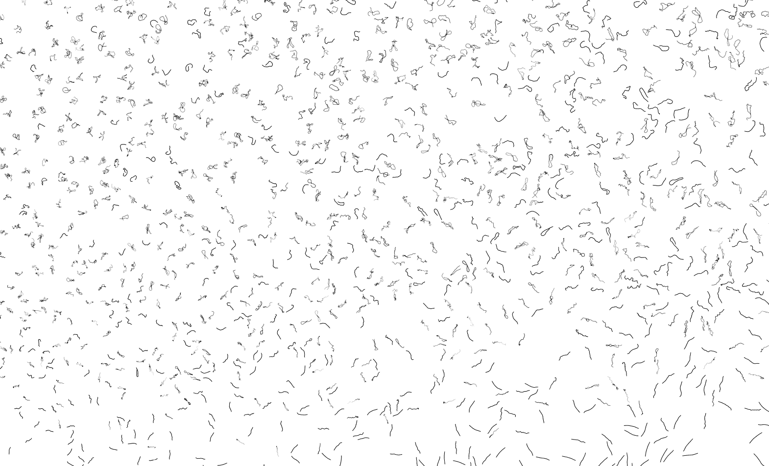
PSFs are obtained by sampling the continuous trajectory TrajCurve (generated by createTrajectory.m) on a regular pixel grid using subpixel linear interpolation. The function createPSFs.m performs such interpolation. Figure 1 illustrates the PFS corresponding to a trajectory curve, while Figure 2 reports some PSFs generated with our functions.
Figure 1: Motion Blur PSFs are obtained by sampling the motion trajectories on a discrete grid using subpixel interpolation.
Figure 2: Motion Blur PSFs are obtained by sampling the motion trajectories on a discrete grid using subpixel interpolation. Observation Model
The image formation model was presented in [Boracchi and Foi 2011] and [Boracchi and Foi 2012], and both the blur due to camera motion and the sensor noise depends on the exposure time.
In particular, two noise terms affect the observations: Figure 3 shows a sequence of images generated with increasing the exposure times.
Figure 3: A sequence of observations generated with the proposed framework. For the sake of visualization images have been rescaled in the [0,1] range, and the corresponding PSF is shown in the upper left corner of each figure (click here to donwload full size picture).
This model provides a unified description of both long-exposure and short-exposure images thus for describing very general acquisition paradigms including the recently proposed approaches based on blurred/noisy image pairs such as [Tico and Vehvilainen 2006] and [Yuan et al 2007]. The function createBlurredRaw.m generate a sequence of blurred/noisy images according to the considered observation model. Codes Description
The Matlab package contains the following functions: Codes Download Matlab Package for Motion Blurred Images References
[Boracchi and Foi, 2012] Modeling the Performance of Image Restoration from Motion Blur
[Boracchi and Foi, 2011] Uniform motion blur in Poissonian noise: blur/noise trade-off
[Tico and Vehvilainen 2006] Estimation of motion blur point spread function from differently exposed image frames
[Yuan et al., 2007] Image deblurring with blurred/noisy image pairs
|


