Playing with conic sections in homogeneous coordinates
Luca Magri. Credits: Prof. Giacomo Boracchi
Contents
Preparation
First, we create an empty image and display it (will be our "canvas")
figure(1)
im=zeros(500,500);
imshow(im, []);
hold on;

Data input: enter five points (then enter)
disp('click 5 points, then enter');
[x, y]=getpts;
scatter(x,y,100,'filled');
click 5 points, then enter

x and y are now column vectors.
x
y
x =

  184.0000
  291.0000
  327.0000
  267.0000
  174.0000


y =

  161.0000
  148.0000
  228.0000
  325.0000
  253.0000
Estimation of conic parameters
using the technique shown in "Multiple View Geometry", page 9. this is equivalent to requiring that the conic passes trhough all the six points
A=[x.^2 x.*y y.^2 x y ones(size(x))]

% A is 5x6: we find the parameter vector (containing [a b c d e f]) as the
% right null space of A.
% This returns a vector N such that A*N=0.  Note that this expresses the
% fact that the conic passes through all the points we inserted.
N = null(A);
% alternatively you can use the svd
[~,~,V] = svd(A);
N = V(:,end);
A =

   1.0e+05 *

    0.3386    0.2962    0.2592    0.0018    0.0016    0.0000
    0.8468    0.4307    0.2190    0.0029    0.0015    0.0000
    1.0693    0.7456    0.5198    0.0033    0.0023    0.0000
    0.7129    0.8677    1.0562    0.0027    0.0032    0.0000
    0.3028    0.4402    0.6401    0.0017    0.0025    0.0000
Let's assign the values to variables and build the 3x3 conic matrix (which is symmetrical)
cc = N(:, 1);
% change the name of variables
[a b c d e f] = deal(cc(1),cc(2),cc(3),cc(4),cc(5),cc(6));
% here is the matrix of the conic: off-diagonal elements must be divided
% by two
C=[a b/2 d/2; b/2 c e/2; d/2 e/2 f]

% Remark: since the right null space has dimension one,
% when the points are taken in general position
% the system admits an infinite number of solutions
% however, these can be expressed as lambda * n, where n
% lambda \in R and n = null(A).
% thus, they all corresponds to the same conic.
C =

    0.0000   -0.0000   -0.0029
   -0.0000    0.0000   -0.0016
   -0.0029   -0.0016    1.0000
Draw the conic
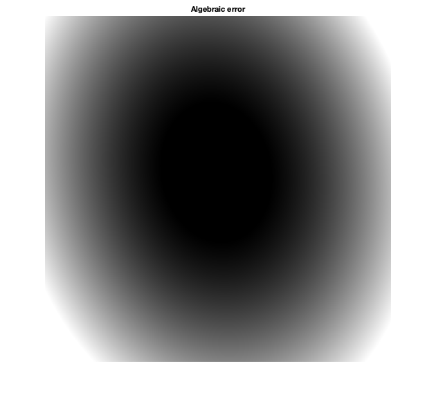
We pick every pixel, and compute the incidence relation.
im=zeros(500,500);
for i=1:500
    for j=1:500
        im(i,j)=[j i 1]*C*[j i 1]'; % this is an algebraic error
    end
end
figure; imshow(im); title('Algebraic error');
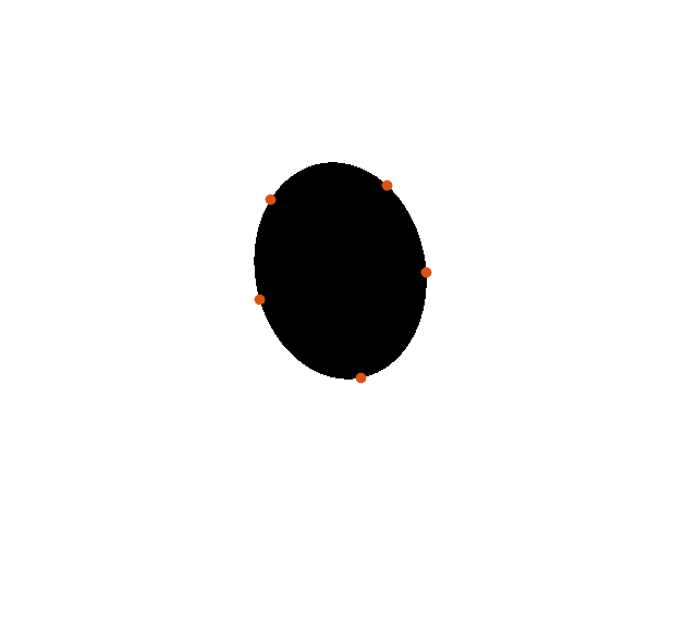
Let's draw black for pixels less than zero, white for pixels greater than 0.
figure(1)
imshow(im > 0);
scatter(x,y, 100, 'filled');
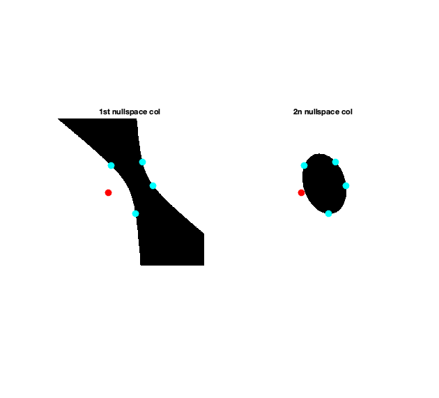
What happen when A is not full rank?
Instead of taking 5 points take just 4 N contains in each column a generator of the null space
N = null(A(1 : 4, :));

% then, any vector living in the null space give rise to a conic
% passing throguh those 4 points. Since the nullspace has dimension two
% we can find two conic passing through the four points
Let's assign the values to variables and build the 3x3 conic matrix (which is symmetrical) Let's start with a first solution, the first vector of the nullspace
cc = N(:, 1);
% cc = N(:, 1) + N(:, 2); % another example, any linear combination is fine
[a, b, c, d, e, f]=deal(cc(1),cc(2),cc(3),cc(4),cc(5),cc(6));
% here is the matrix of the conic
C1_four =[a b/2 d/2; b/2 c e/2; d/2 e/2 f]
% Let's consider a second solution, the second  vector of the nullspace
cc = N(:, 2);
% cc = N(:, 1) + 2*N(:, 2); % another example, any linear combination is fine
[a, b, c, d, e, f]=deal(cc(1),cc(2),cc(3),cc(4),cc(5),cc(6));
% here is the matrix of the conic
C2_four =[a b/2 d/2; b/2 c e/2; d/2 e/2 f]
C1_four =

    0.0024   -0.0015   -0.3198
   -0.0015    0.0002    0.3844
   -0.3198    0.3844   -0.0023


C2_four =

    0.0000   -0.0000   -0.0032
   -0.0000    0.0000   -0.0012
   -0.0032   -0.0012    1.0000
Draw the conic
We pick every pixel, and compute the incidence relation.
im_four=zeros(500,500);
for i=1:500
    for j=1:500
        im_four1(i,j)=[j i 1]*C1_four*[j i 1]';
        im_four2(i,j)=[j i 1]*C2_four*[j i 1]';
    end
end

figure(2)
subplot(1,2,1)
imshow(im_four1>0);
hold on;
scatter(x(1 : 4), y(1 : 4), 100, 'filled','cyan');
scatter(x(5), y(5), 100, 'filled','red');
title('1st nullspace col ')
subplot(1,2,2)
imshow(im_four2>0);
hold on
scatter(x(1 : 4), y(1 : 4), 100, 'filled','cyan');
scatter(x(5), y(5), 100, 'filled','red');
title('2n nullspace col ')
hold off
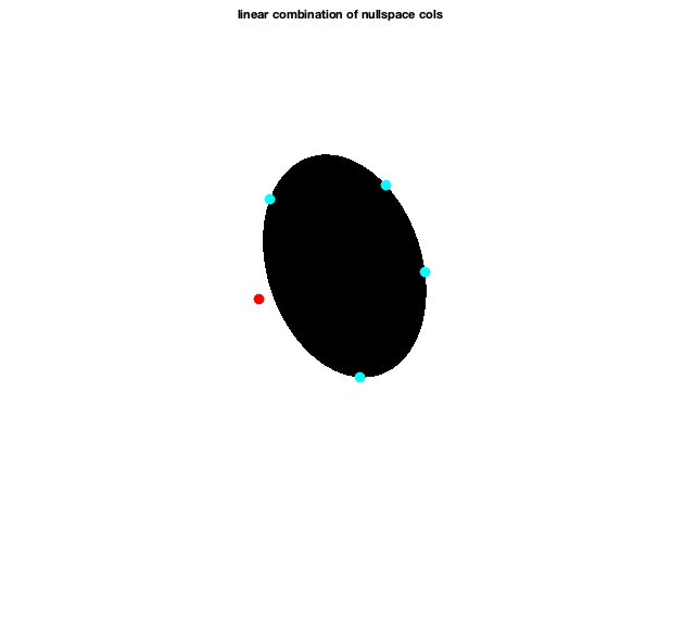
Any linear combination of N1 and N2 is a solution
we can draw a pencil of conics
for lambda = [10, 200, 3000, 100000]

    cc = 1*N(:,1)+ lambda*N(:,2);
    [a, b, c, d, e, f]=deal(cc(1),cc(2),cc(3),cc(4),cc(5),cc(6));
    C3_four =[a b/2 d/2; b/2 c e/2; d/2 e/2 f];
    % We pick every pixel, and compute the incidence relation.
    im_four=zeros(500,500);
    for i=1:500
        for j=1:500
            im_four3(i,j)=[j i 1]*C3_four*[j i 1]';
        end
    end
    figure(3)
    imshow(im_four3>0);
    hold on;
    scatter(x(1 : 4), y(1 : 4), 100, 'filled','cyan');
    scatter(x(5), y(5), 100, 'filled','red');
    title('linear combination of nullspace cols ')
    pause;
end
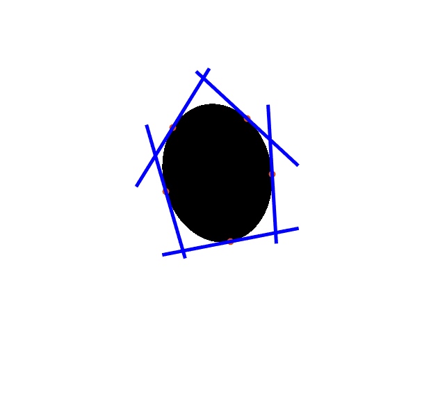
Tangent lines
Let's draw the tangents to our points: the tangent line in homogeneous coordinates is l the line tangent to C at the line x is defined as l = C*x
% this is the line tangent to the first point
l1 = C * [x(1); y(1); 1];
% here I compute all the tangent lines simultaneously
% stacking all the vectors in the columns of the matrix l
l=C*[x y ones(size(x))]'
l =

   -0.0007    0.0006    0.0010    0.0001   -0.0010
   -0.0005   -0.0007   -0.0001    0.0008    0.0003
    0.2114   -0.0796   -0.3101   -0.2878    0.0960
in order to draw it we find its angle, then plot a line of length 200 around it. In order to write less lines of code, I'm doing a bit of hacks with matrices and vectors here: theta will be a column vector of angles, and with a single plot command I'll plot all the lines. Check out the documentation of plot to understand what's happening.
theta=atan2(-l(1,:),l(2,:));
theta = theta';
figure(1), hold on
plot([x-cos(theta)*100 x+cos(theta)*100]',...
    [y-sin(theta)*100 y+sin(theta)*100]','b-','LineWidth',5);
Let's compute the dual conic and check that all the tangent lines we computed previously actually satisfy the relation (up to numeric precision issues).
Cstar=inv(C);
l(:,1)'*Cstar*l(:,1)
l(:,2)'*Cstar*l(:,2)
l(:,3)'*Cstar*l(:,3)
l(:,4)'*Cstar*l(:,4)
l(:,5)'*Cstar*l(:,5)
ans =

   2.7756e-16


ans =

   5.8287e-16


ans =

   3.3307e-16


ans =

  -4.4409e-16


ans =

  -4.9960e-16