stitch

A naive way to stitch two images
Data entry
Homography estimation using our codes
Let's see the result
Let's try to see both the images
blend the images
Homography estimation
Transformations
Visualizations
Notes

A naive way to stitch two images

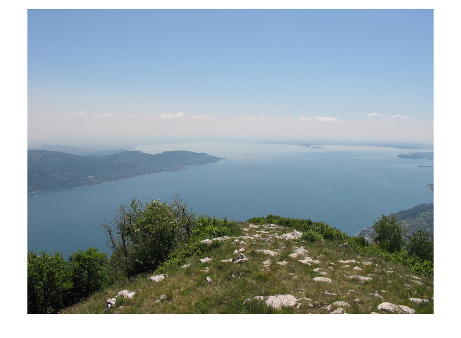
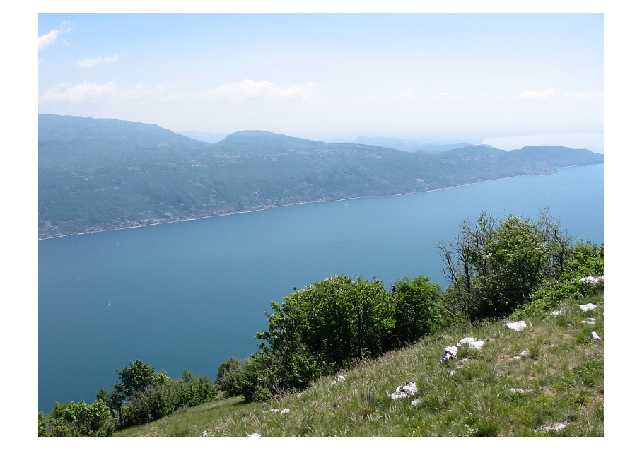
Let's load a pair of images, taken from the same point of view. We want to stitch them.

close all
clc
addpath('../')

im1=imread('im1.jpg');
im2=imread('im2.jpg');
im1f=figure; imshow(im1);
im2f=figure; imshow(im2);

Data entry

We manually :-( pick four points in the first image, and four corresponding points on the second image

figure(im1f), [x1,y1]=getpts
figure(im1f), hold on, plot(x1,y1,'oy', 'LineWidth', 5, 'MarkerSize', 10);
figure(im2f), [x2,y2]=getpts
figure(im2f), hold on, plot(x2,y2,'oy', 'LineWidth', 5, 'MarkerSize', 10);

Homography estimation using our codes

a = [x1(1); y1(1); 1];
b = [x1(2); y1(2); 1];
c = [x1(3); y1(3); 1];
d = [x1(4); y1(4); 1];
X = [a, b, c, d];

ap = [x2(1); y2(1); 1];
bp = [x2(2); y2(2); 1];
cp = [x2(3); y2(3); 1];
dp = [x2(4); y2(4); 1];
XP = [ap, bp, cp, dp];


% apply preconditioning to ease DLT algorithm
% Tp and TP are similarity trasformations
[pCond, Tp] = precond(X);
[PCond, TP] = precond(XP);

% estimate the homography among transformed points
Hc = homographyEstimation(pCond, PCond);

% adjust the homography taking into account the similarities
H = inv(TP) * Hc * Tp; % the trasnformation to be applied

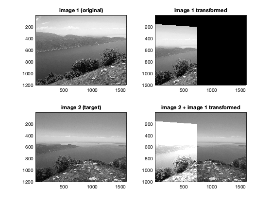
Let's see the result

% apply the homography to the red channel of the first image
% J is the transformed image rendered in a canvas with the same dimension
% of image2
J = imwarpLinear(im1(:,:,1), H, [1, 1, 1600, 1200]);

figure(23);
subplot(2,2,1)
imagesc(im1(:,:,1)), title('image 1 (original)'), colormap gray;
subplot(2,2,2)
imagesc(J), title('image 1 transformed'), colormap gray;
subplot(2,2,3)
imagesc(im2(:,:,1)), title('image 2 (target)'), colormap gray;
subplot(2,2,4)
imagesc(im2(:,:,1)+ uint8(J)), title('image 2 + image 1 transformed'), colormap gray;
% we have lost part of the image content using imwarplinear!

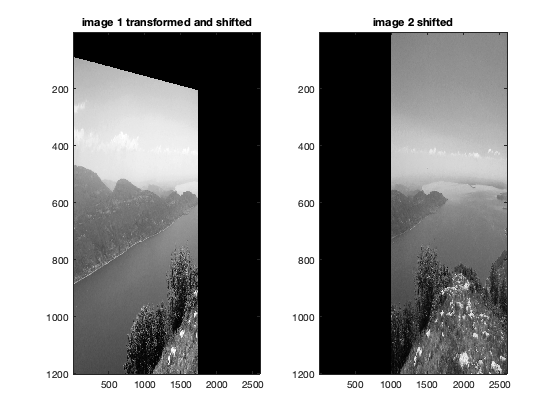
Let's try to see both the images

% create an homography that shift the image to the right
shift = 1000;
H2 = [1 0 shift; 0 1 0; 0 0 1];
im2_shifted = imwarpLinear(im2(:,:,1), H2, [1, 1, size(im2,2) + shift, size(im2,1)]);

% now we have to transform im1 and we need to account for the shifting
J_shifted = imwarpLinear(im1(:,:,1), H2*H, [1, 1, size(im2,2) + shift, size(im2,1)]);
figure(26)
subplot(1,2,1)
imagesc(J_shifted), title('image 1 transformed and shifted'), colormap gray;
subplot(1,2,2)
imagesc(im2_shifted), title('image 2 shifted'), colormap gray;

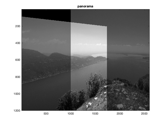
blend the images

figure(225), imagesc(J_shifted + im2_shifted), title('panorama'), colormap gray;

Homography estimation

The matlab maketform function returns an homography given four points and their transformed ones, which is the minimal information which defines an homography. A naive algorithm which solves this problem is in "Multiple View Geometry", page 35. Better algorithms are in chapter 4 of the same book.

T=maketform('projective',[x2 y2],[x1 y1]);
T.tdata.T

ans =

    0.7130   -0.0620   -0.0002
   -0.0055    0.9175   -0.0000
  859.3463 -141.2110    1.0000

this is the computed homography, a 3x3 matrix. It transforms the second image to match the first.

Transformations

Let's not transform the images, and place both on the same reference frame. There are some hacks with xdata and ydata here, check the imtransform docs if you are interested in the details.

[im2t,xdataim2t,ydataim2t]=imtransform(im2,T);
% now xdataim2t and ydataim2t store the bounds of the transformed im2
xdataout=[min(1,xdataim2t(1)) max(size(im1,2),xdataim2t(2))];
ydataout=[min(1,ydataim2t(1)) max(size(im1,1),ydataim2t(2))];
% let's transform both images with the computed xdata and ydata
im2t=imtransform(im2,T,'XData',xdataout,'YData',ydataout);
im1t=imtransform(im1,maketform('affine',eye(3)),'XData',xdataout,'YData',ydataout);

Visualizations

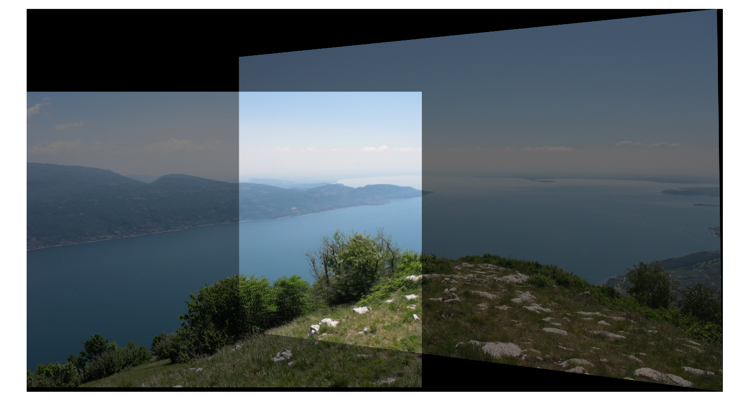
now im1t and im2t are equal-size images ready to be merged. Let's average them

ims=im1t/2+im2t/2;
figure, imshow(ims)

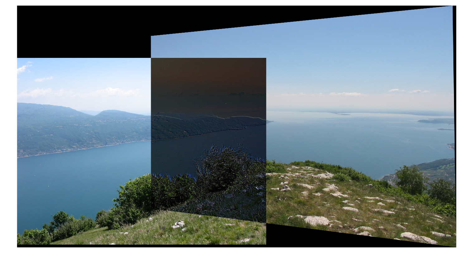
if we want to better analyze the match quality, let's compute the difference of the two images and look at the absolute value

imd=uint8(abs(double(im1t)-double(im2t)));
% the casts necessary due to the images' data types
imshow(imd);

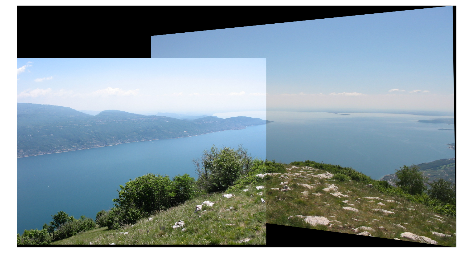
you can get a decent composite by picking the maximum at each pixel: however, note that the seam is visible, because the exposure in the two images is not equal. Real stitching software compensates for this.

ims=max(im1t,im2t);
imshow(ims);

Notes

real stitching software do a lot more than this. And, they pick matching points automatically. :-) The full panorama (which is from Cima Comer, on Lago di Garda) is found here: http://www.leet.it/home/lale/files/Garda-pano.jpg It was made using Hugin and panotools: http://hugin.sourceforge.net/ Note that exposure has been compensated between images. Also, curved image boundaries suggest that not only homographies were compensated to rectify the image, but also higher-order distorsions.

Contents