Contents

% Giacomo Boracchi
% course Computer Vision and Pattern Recognition, USI Spring 2020
%
% February 2020

close all
clear
clc
addpath(genpath('C:\Users\Giacomo Boracchi\Dropbox (DEIB)\Didattica\2020_Computer_Vision_Pattern_Recognition_USI\Materiali\Zisserman_Codes\VGG-Multiple-View-Geometry-master'));
FNT_SZ = 28;
I = imread('projgeomfigs-chapel.png');
% I = imread('rubiks-cube-1390088_1920.jpg');
I = im2double(rgb2gray(I)); % move to RGB since image transformations have been implented over grayscale images

Warning: Too many
IDAT's found.
The image data
may be corrupt. 

Select a few points to be rectified

figure(1), imshow(I);
hold on;
[x, y] = getpts();
a = [x(1); y(1); 1];
b = [x(2); y(2); 1];
c = [x(3); y(3); 1];
d = [x(4); y(4); 1];

text(a(1), a(2), 'a', 'FontSize', FNT_SZ, 'Color', 'b')
text(b(1), b(2), 'b', 'FontSize', FNT_SZ, 'Color', 'b')
text(c(1), c(2), 'c', 'FontSize', FNT_SZ, 'Color', 'b')
text(d(1), d(2), 'd', 'FontSize', FNT_SZ, 'Color', 'b')

OPTION2: estimate the trasformation mapping 4 points over a square

X = [a, b, c, d];
aP = [1; 1; 1];
bP = [1; 500; 1];
cP = [500; 500; 1];
dP = [500; 1; 1];
XP = [aP, bP, cP, dP];

% estimate homography using DTL algorithm
H = homographyEstimation(X, XP);

% Apply the trasformation to the image mapping pixel centers using H^-1 and bilinear interpolation
J = imwarpLinear(I, H, [1, 1, 1500, 1500]);

figure, imagesc(J), colormap gray, axis equal;

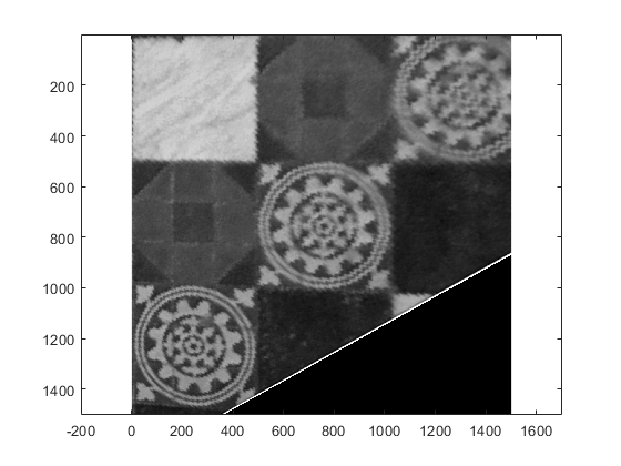
OPTION 2BIS: estimate the transformation by preconditioning points first

% apply preconditioning to ease DLT algorithm
% Tp and TP are similarity trasformations
[pCond, Tp] = precond(X);
[PCond, TP] = precond(XP);

% estimate the homography among transformed points
Hc = homographyEstimation(pCond, PCond);

% adjust the homography taking into account the similarities
H = inv(TP) * Hc * Tp; % the trasnformation to be applied

% Apply the trasformation to the image
J = imwarpLinear(I, H, [1, 1, 1500, 1500]);
figure, imagesc(J), colormap gray, axis equal;

Published with MATLAB® R2017b