drawcube

A simple geometrical construction with 2D homogeneous coordinates
Data input
Finding and plotting vanishing points
Finding the missing points (d and e)
Drawing
Rectify a face

A simple geometrical construction with 2D homogeneous coordinates

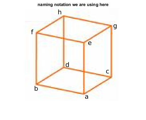
Our goal is to complete the drawing of a cuboid. We use need six vertices on the contour of the cuboid.

credits Alessandro Giusti alessandrog@idsia.ch

Giacomo Boracchi December 12, 2016

close all
clear
clc

Data input

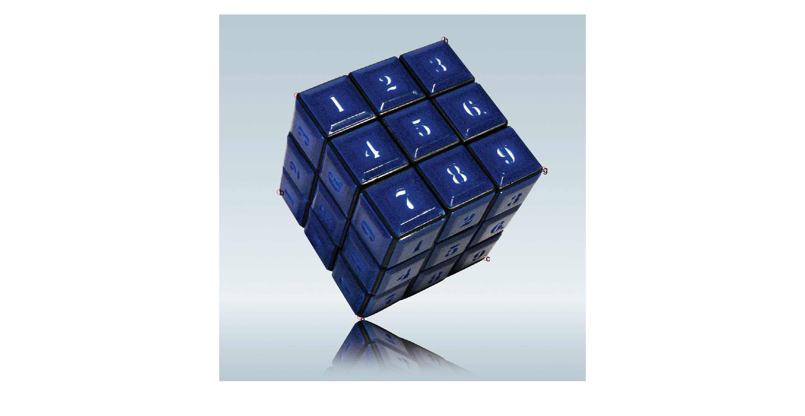
FNT_SZ = 20;
im=imread('bluecube.jpg');
figure(1), imshow(im);
% keeps on drawing multiple elements on the same figure
hold on;
% select six visible verteces of the cube
[x y]=getpts;
plot(x,y,'or','MarkerSize',12);

% take the points in homogenous coordinates
a=[x(1) y(1) 1]';
text(a(1), a(2), 'a', 'FontSize', FNT_SZ, 'Color', 'w')
b=[x(2) y(2) 1]';
text(b(1), b(2), 'b', 'FontSize', FNT_SZ, 'Color', 'w')
f=[x(3) y(3) 1]';
text(f(1), f(2), 'f', 'FontSize', FNT_SZ, 'Color', 'w')
h=[x(4) y(4) 1]';
text(h(1), h(2), 'h', 'FontSize', FNT_SZ, 'Color', 'w')
g=[x(5) y(5) 1]';
text(g(1), g(2), 'g', 'FontSize', FNT_SZ, 'Color', 'w')
c=[x(6) y(6) 1]';
text(c(1), c(2), 'c', 'FontSize', FNT_SZ, 'Color', 'w')

figure(2), imshow(imread('simplecube-letters.png')), title('naming notation we are using here');

% call figure 1 back (we have to draw on this)
figure(1),

Warning: Image is too big to fit on
screen; displaying at 50%

Finding and plotting vanishing points

lAB= cross(A,B) where A and B are points computes the line lAB passing through AB (the 3 coefficient vector)

D = cross(lAB, lGH), where lAB and lGH are the 1x3 coefficient vectors yield the intersection of the two lines

to determine wether a point A belongs to a line l it's enough to check whether the scalar product between A and l is zero, i.e., A' * l == 0

vab=cross(cross(a,b),cross(h,g));
vac=cross(cross(a,c),cross(f,h));
vae=cross(cross(b,f),cross(c,g));

% points have to be normalized before visualizing them on the plane
vab=vab/vab(3);
vac=vac/vac(3);
vae=vae/vae(3);

% these are quite far from the image region
plot(vab(1),vab(2),'x');
plot(vac(1),vac(2),'x');
plot(vae(1),vae(2),'x');

Finding the missing points (d and e)

d=cross(cross(b,vac),cross(c,vab));
d=d/d(3);
e=cross(cross(g,vac),cross(f,vab));
e=e/e(3);

Drawing

we can now finally draw the cube.

myline=[a';b';d';c';a'];
line(myline(:,1),myline(:,2),'LineWidth',5);
myline=[e';f';h';g';e'];
line(myline(:,1),myline(:,2),'LineWidth',5);
myline=[a';e'];
line(myline(:,1),myline(:,2),'LineWidth',5);
myline=[b';f'];
line(myline(:,1),myline(:,2),'LineWidth',5);
myline=[c';g'];
line(myline(:,1),myline(:,2),'LineWidth',5);
myline=[d';h'];
line(myline(:,1),myline(:,2),'LineWidth',5);

Rectify a face

We can also transform the image so that a face becomes a square.

T = maketform('projective',[a(1:2)';b(1:2)';f(1:2)';e(1:2)'],[0 0;300,0;300,300;0,300]);
figure, imshow(imtransform(im,T));

Warning: Image is too big to fit on
screen; displaying at 33%

Such transformation is called homography, and will be presented later during the Image Analysis and Synthesis course. Still, it is a linear transformation, so it has the same form of the simpler 2D transformations (translations and rotations) which have already been introduced, a 3x3 matrix:

T.tdata.T