Contents

Some examples of digital filters for images

Giacomo Boracchi

close all
clear
clc

notation

% I  original image
% h  LTI discrete filter
% G  convolution output
% n  noise
% z  noisy observation

Linear Filters

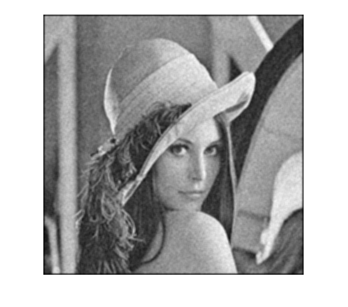
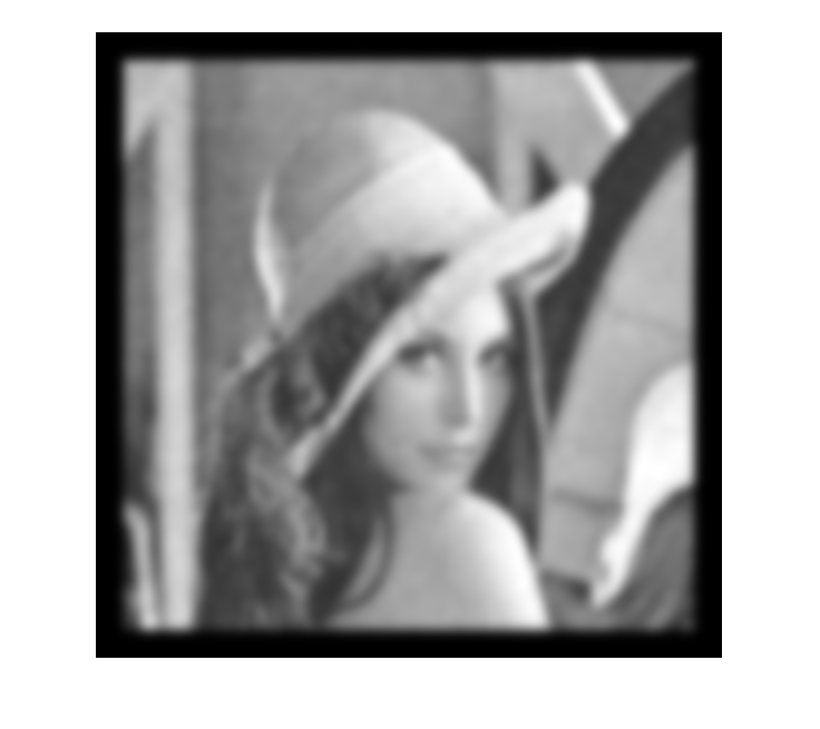
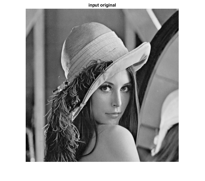
FILTER_SIZE = 21;

% load image  check the filename!!
I = im2double(imread('image_lena512.png'));
figure(1), imshow(I, []), title('I, original image')

% have a look at the image size
whos I

% create averaging filter
h = ones(FILTER_SIZE)/(FILTER_SIZE^2);

% generate "averaged" image
G = conv2(I, h);

% have a look at size of convolution
whos G

G = conv2(I, h, 'same');

% use the option same to keep image size constant
whos G

% display the original image and the distribution of pixel intensities
figure(1), imshow(I,[]),title('input original')
figure(2), imshow(G,[]),title('convolved output')

% generate "averaged" image
z2 = conv2(h, I, 'same');

% display the original image and the distribution of pixel intensities
figure(1), imshow(I,[]),title('input original')
figure(2), imshow(G,[]),title('convolved output')

  Name        Size               Bytes  Class     Attributes

  I         512x512            2097152  double              

  Name        Size               Bytes  Class     Attributes

  G         532x532            2264192  double              

  Name        Size               Bytes  Class     Attributes

  G         512x512            2097152  double              

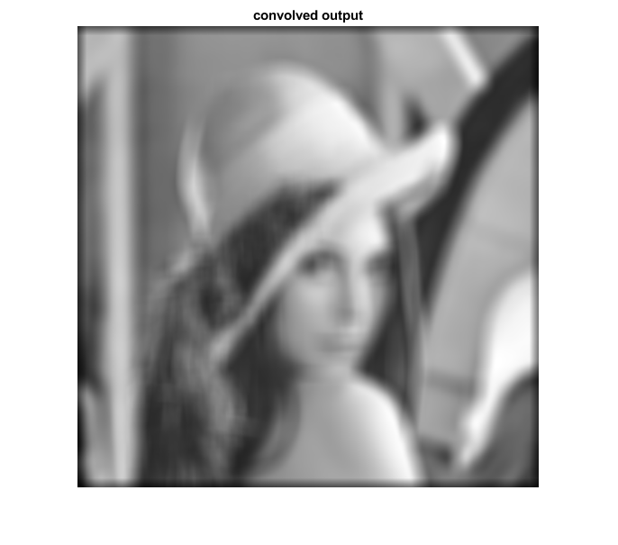
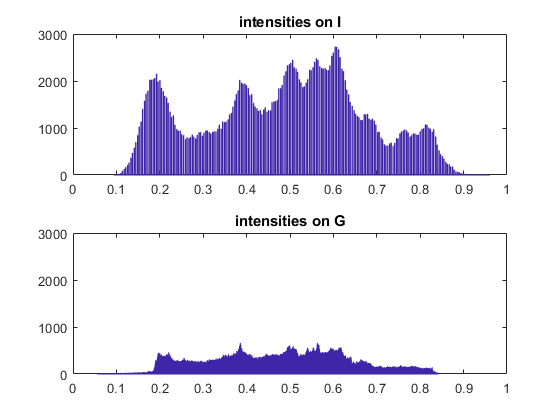
While intensities of I are values like {i/255, i = 0,.., 255} there are much more values in G thanks to the local smoothing

figure(4),
subplot(2,1,1), hist(I(:) , 1000), title('intensities on I'), axis([0 1 0 3000])
subplot(2,1,2), hist(G(:) , 1000), title('intensities on G'), axis([0 1 0 3000])

shift filter

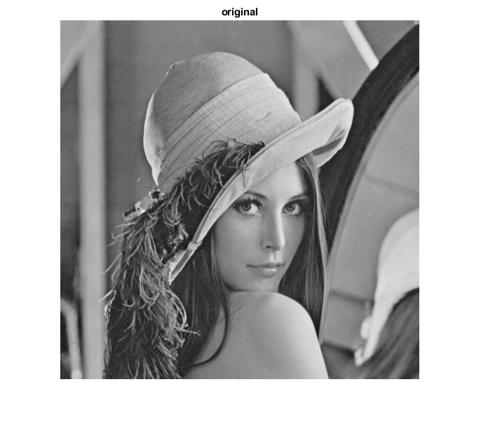
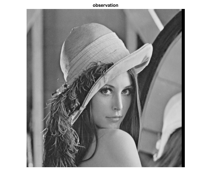
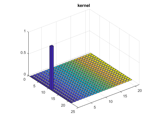
FILTER_SIZE = 21;
h=zeros(FILTER_SIZE );
h((FILTER_SIZE  - 1) / 2 + 1 ,1) = 1;

G=conv2(I, h, 'same');

% display
figure(1), imshow(I),title('original')
figure(2), imshow(G),title('observation')
figure(3), bar3(h),title('kernel')

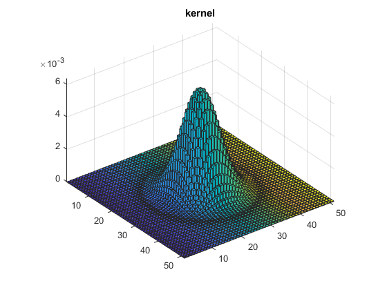
Gaussian Filters

h_size = 51;
sigma_gauss = 5;
h = fspecial('gaussian' , h_size , sigma_gauss);
figure(3),bar3(h),title('kernel')

G=conv2(I , h , 'same');

% display
figure(1), imshow(I),title('original')
figure(2), imshow(G),title('observation')
figure(3), bar3(h),title('kernel')

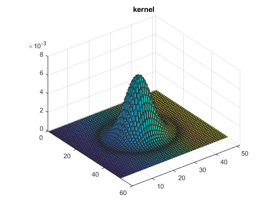
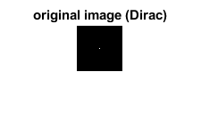
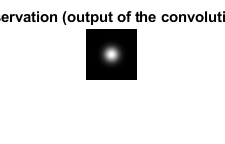
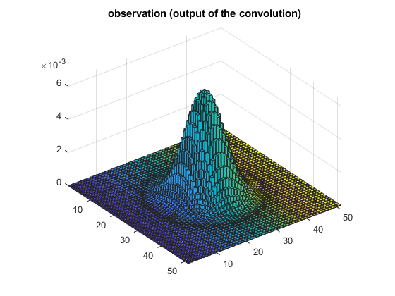
The impulse response of a filter can be computed as the convolution against a Dirac

close all

I = zeros(51);
I(26 , 26) = 1;

G=conv2(I , h , 'same');

% display
figure(1), imshow(I),title('original image (Dirac)')
figure(2), imshow(G, []), title('observation (output of the convolution)')
figure(3), bar3(G),title('observation (output of the convolution)'), axis tight
% check that it corresponds to the kernel
figure(4), bar3(h),title('kernel'), axis tight

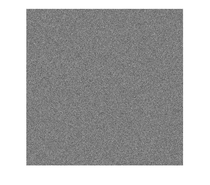
Generating a noisy image as an image corrupted by additive Gaussian white noise

I=im2double(imread('image_lena512.png'));
figure(1), imshow(I,[]),title('I, original image')

sigma_noise = 0.1;

% the noise is a matrix having the same sizes of the original image
n = sigma_noise * randn(size(I));
figure(4), imshow(n, [])

% Additive White Gaussian Noise  (AWGN): the noisy observation is given by
z = I + n;
figure(5),imshow(G);

denoising via smoothing (see slides and possibly LASIP package)

% suppress noise by averaging: each pixel is replaced by the average over a 7x7 neighboor, uniform weight
figure(6),imshow(conv2(z, ones(5)/(5^2)),[])

% suppress noise by averaging: each pixel is replaced by the average over a neighbor defined by the Gaussian kernel,
% which also defines the averaging weights
figure(7),imshow(conv2(z, h),[])

Published with MATLAB® R2017b