Contents

Quick primer on some insightful characteristics of matlab for the course

MATlab : Matrix Laboratory can be used as a scripting language any variable is a matrix (a scalar is a special case of a multidimensional array)

credits Alessandro Giusti alessandrog@idsia.ch

Giacomo Boracchi September 25, 2017

close all
clear
clc

disp('For enquiry, please send an email to giacomo.boracchi@polimi.it');

% variables are defined by an assignement
v=3
size(v)

% data types are automatically defined depending on the assigned value
whos v

% a row vector (commas can be omitted)
r=[1, 2, 3, 4]
size(r)

% a column vector
c=[1; 2; 3; 4]
size(c)

% a matrix
v=[1 2; 3 4]
size(v)

% you can concatenate matrices or vectors as far as their size are consistent
B=[v', v']

C = [v ; v]

% this is not allowed
% K = [r,c]

For enquiry, please send an email to giacomo.boracchi@polimi.it

v =

     3


ans =

     1     1

  Name      Size            Bytes  Class     Attributes

  v         1x1                 8  double              


r =

     1     2     3     4


ans =

     1     4


c =

     1
     2
     3
     4


ans =

     4     1


v =

     1     2
     3     4


ans =

     2     2


B =

     1     3     1     3
     2     4     2     4


C =

     1     2
     3     4
     1     2
     3     4

subarray

v(indexes) returns a vector of all the elements of v at locations in array indexes

% you can reference single or multiple values in an array:
v(1,2) % first row and second column (row and column indices are 1-based)
v(:,2) % the second column of v
v(1,:) % the first row
B(:,2:4) % some of the columns
v(5,5) = 10 % you can extend vectors / matrices by assigning some element our of the range

ans =

     2


ans =

     2
     4


ans =

     1     2


ans =

     3     1     3
     4     2     4


v =

     1     2     0     0     0
     3     4     0     0     0
     0     0     0     0     0
     0     0     0     0     0
     0     0     0     0    10

operation on vectors are from linear algebra

common operations work on matrices (careful about multiplication and division)

v*v'

ans =

     5    11     0     0     0
    11    25     0     0     0
     0     0     0     0     0
     0     0     0     0     0
     0     0     0     0   100

there are also element-wise operators

[1 2 3].*[4 5 6]

[1 2 3] + 5
[1 2 3] * 2 % no need to use element-wise operator with scalars
[1 2 3] .* 2 %explicit element-wise multiplication
[1 2 3] / 2
[1 2 3] ./ 2 %explicit element-wise division
[1 2 3] .^ 2 %explicit element-wise power


[1 2 3] * [4 5 6]' % this matrix product, returns a scalar (it is the inner product)

[1 2 3]' * [4 5 6] % this is the matrix product, returns a 3 x 3 matrix

ans =

     4    10    18


ans =

     6     7     8


ans =

     2     4     6


ans =

     2     4     6


ans =

    0.5000    1.0000    1.5000


ans =

    0.5000    1.0000    1.5000


ans =

     1     4     9


ans =

    32


ans =

     4     5     6
     8    10    12
    12    15    18

variables have datatypes (usually you can forget, but not when dealing with images). Most common types we will consider are double, (i.e. double-precision floating point), uint8 (i.e. unsigned integers with 8 bits, [0 255] range), logical (i.e. boolean).

whos v

%
% casting to 8-bit integers
v = uint8(v)
whos v

  Name      Size            Bytes  Class     Attributes

  v         5x5               200  double              


v =

    1    2    0    0    0
    3    4    0    0    0
    0    0    0    0    0
    0    0    0    0    0
    0    0    0    0   10

  Name      Size            Bytes  Class    Attributes

  v         5x5                25  uint8              

logicals

you can compare a vector via the customary relational operator and obtain a vector of logicals

v=v>2
whos v

v =

     0     0     0     0     0
     1     1     0     0     0
     0     0     0     0     0
     0     0     0     0     0
     0     0     0     0     1

  Name      Size            Bytes  Class      Attributes

  v         5x5                25  logical              

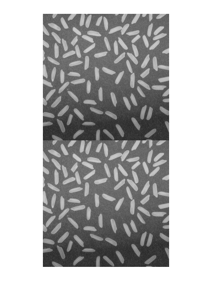
Images are matrices

im=imread('rice.png');
whos im
%
%
imshow(im);
%
%
imshow([im im]);
%
%
imshow([im; im]);

  Name        Size             Bytes  Class    Attributes

  im        256x256            65536  uint8              

Matrices are images

M = rand(100);
% M = eye(100);
imshow(M);
%
%
% imshow(magic(200),[])

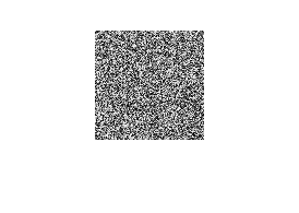
... but datatype matters! Careful about data range: [0 1] for double and logical, [0 255] for uint8

imshow(double(im));
%
%
imshow(double(im)/255);
%
%
imshow(uint8(double(im)/255));

plot the image histogram

compute histogram of image intensity values

h = hist(im(:), [0: 255]);
figure(2), stairs([0: 255], h), title('intensity histogram')
axis tight

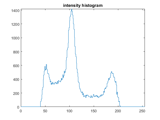
Image brigthness can be modified by adding an offset to each pixel

figure(1), imshow(im + 50), title('brigthness increases of 50 graylevels');
% few pixels are saturated
figure(1), imshow(im + 100), title('brigthness increases of 100 graylevels');

% contrast can be modified by streching the histogram, image has to be
% converted in double format
eq = double(im - min(im(:)))/double(max(im(:)) - min(im(:))) * 255;

figure(1), imshow(uint8(eq), []), title('Image now covers the whole range');

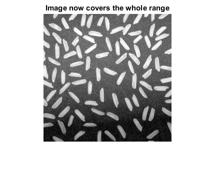
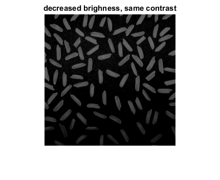
Image ranges (in the visualization) can be also controlled by the second argument to imshow

imshow(im,[-100 156]); title('increased brighness same contrast');
%
imshow(im,[0 156]); title('increased brighness and contrast');
%
imshow(im,[ 100 256]); title('decreased brighness, increased contrast');
%
imshow(im,[ 100 356]); title('decreased brighness, same contrast');
%
% Consider that brightness and contrast can be also changed by
% - adding an offset or
% - scaling the image

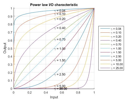
gamma correction

a nonlinear transformation used to change the contrast in different range of intensities

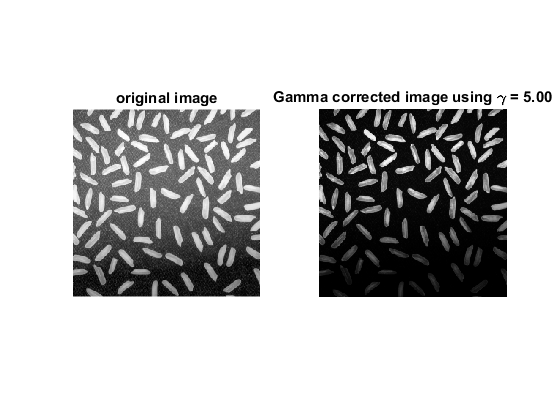
figure(3);
cla
hold on;
x = 0:0.001:1;
for gamma = [.04 .1 .2 .4 .7 1 1.5 2.5 5 10 25]
    y = x.^gamma;
    plot(x,y,'DisplayName',sprintf('\\gamma = %.2f',gamma));
    % display the text
    text(x(round(end/2)),y(round(end / 2)), sprintf('\\gamma = %.2f',gamma));
end
xlabel('Input');
ylabel('Output');
title('Power law I/O characteristic');
leg = legend('Location','eastoutside');
axis equal
grid on
hold off

% play with gammaVal and set a different value for the gamma Correction.
% check which part of the image are being mostly affected by this transformation
gammaVal = 5;
imd = im2double(im);
figure(4)
subplot(1,2,1)
imshow(imd, [])
title('original image')
subplot(1,2,2)
imshow(imd.^gammaVal, [])
title(sprintf('Gamma corrected image using \\gamma = %.2f', gammaVal));

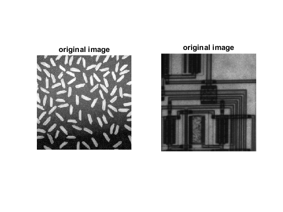
It's also useful to play with the imtool command and its "contrast" function, which also shows the histogram of the image.

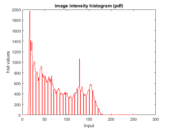
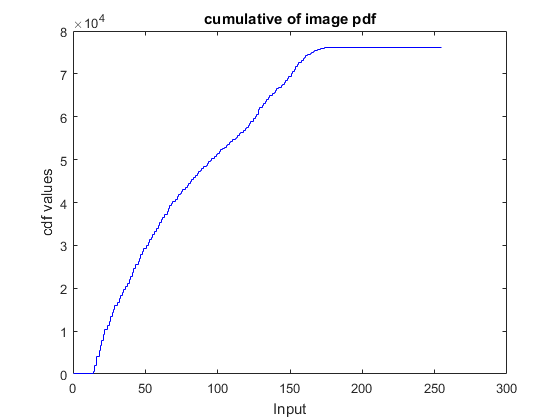
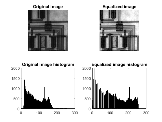
a = imread('circuit.tif');
figure(4), imshow(a), title('original image');

% compute the histogram of all the intensities
hist_a = hist(a(:), [0 : 255]);
figure(5),
stairs([0 : 255], hist_a, 'r'), title('image intensity histogram (pdf)')
xlabel('Input');
ylabel('hist values');

% the histogram can be computed also as
% imhist(a);

% the histogram can be seen as the pdf of a RV corresponding to pixel realization
% histogram equalization consists in applying a monotonic transformation
% that brings this pdf towards a uniform distribution.

% this trasformation is x -> CDF(hist, x) where
% CDF is the cumulative density function of the histogram
% x is the intensity of a pixel
cdf_a = cumsum(hist_a);

cdf_a_map = uint8(cdf_a / cdf_a(end) * 255);

figure(6),
stairs([0 : 255], cdf_a, 'b'), title('cumulative of image pdf')
xlabel('Input');
ylabel('cdf values');


a_eq = cdf_a_map(a + 1);

hist_a_eq = hist(a_eq(:), 0 : 256);


figure(8);
subplot(2,2,1);
imshow(a);
title('Original image');

subplot(2,2,2);
imshow(a_eq);
title('Equalized image');

subplot(2,2,3);
bar(hist_a);
title('Original image histogram');

subplot(2,2,4);
bar(hist_a_eq);
title('Equalized image histogram');

Color is represented by 3 channels (RGB)

You get a 3d matrix

im=imread('bluecube.jpg');
whos im
figure()
imshow(im);

  Name         Size                  Bytes  Class    Attributes

  im        1417x1417x3            6023667  uint8              

Warning: Image is too big to fit on screen; displaying
at 50% 

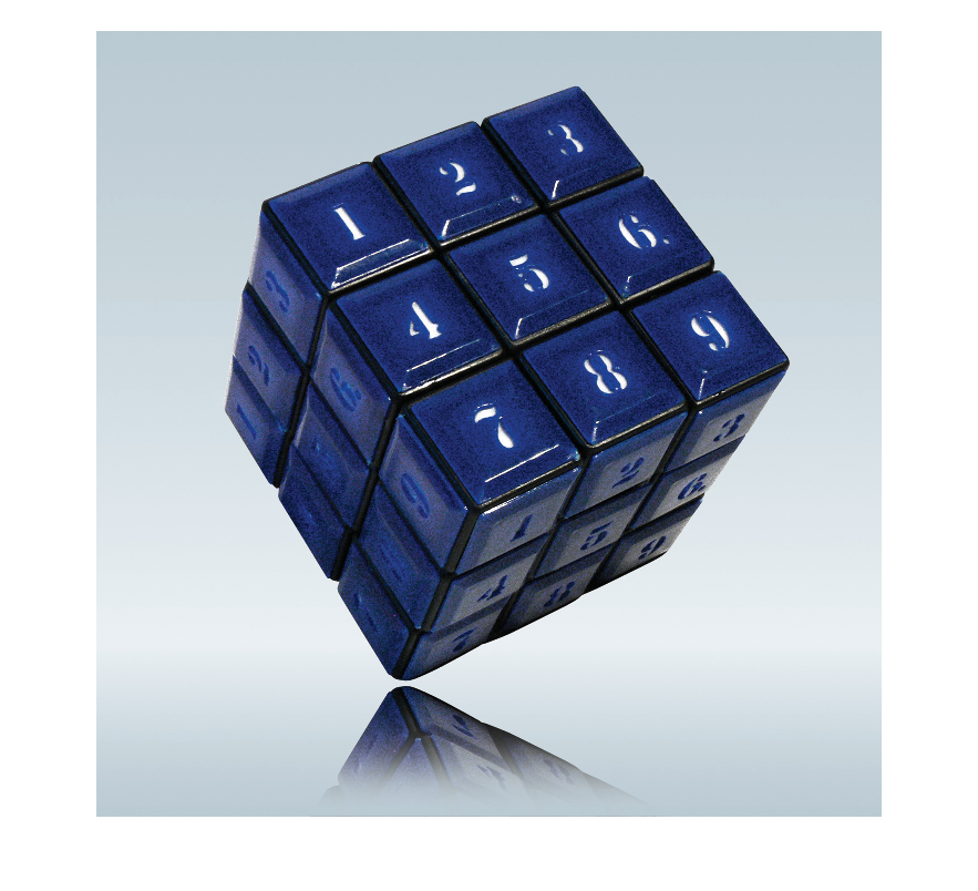
this is a 3D matrix, because it has 3 dimensions (not because the 3rd dimension has only 3 elements).

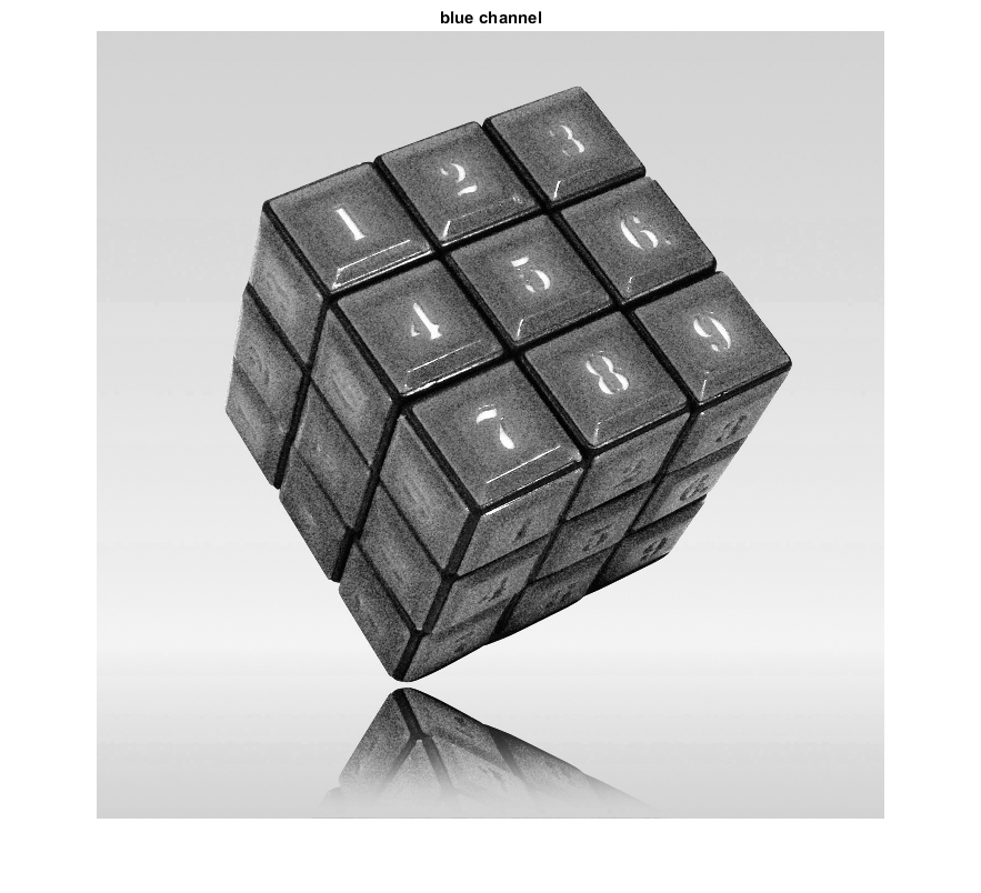
test=im(:,:,1:2);
whos test

%
% We can instead see each single channel as a grayscale image
imr=im(:,:,1);
whos imr % note: now it's 2D, so it will be displayed as grayscale
%
%
imshow(imr), title('red channel')
%
%
img=im(:,:,2);
imshow(img), title('green channel')
%
%
imb=im(:,:,3);
imshow(imb), title('blue channel')

  Name         Size                  Bytes  Class    Attributes

  test      1417x1417x2            4015778  uint8              

  Name         Size                Bytes  Class    Attributes

  imr       1417x1417            2007889  uint8              

Warning: Image is too big to fit on screen; displaying
at 50% 
Warning: Image is too big to fit on screen; displaying
at 50% 
Warning: Image is too big to fit on screen; displaying
at 50% 

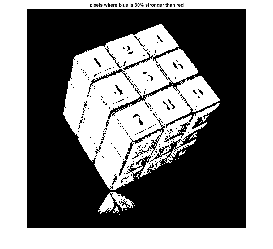
logicals

We can plot the result of logical operations

l=imb>(1.3*imr);
whos l
%
%
imshow(l); title('pixels where blue is 30% stronger than red');

  Name         Size                Bytes  Class      Attributes

  l         1417x1417            2007889  logical              

Warning: Image is too big to fit on screen; displaying
at 50% 

Published with MATLAB® R2015b