Edge Detection

Giacomo Boracchi

Contents

close all
clear
clc

Building filters as smoothing + differentiating filters

disp('differentiating filters')
diffx=[1 -1]
diffy = diffx'

%smoothing filters Previtt
sx=ones(2,3);
sy=sx';

% build Previtt derivative filters
disp('derivative filters Previtt')
dx=conv2(sy , diffx)
dy=conv2(sx , diffy)

%smoothing filters Sobel
sx=[1 2 1 ; 1 2 1];
sy=sx';

% Build Sobel derivative filters
disp(' derivative filters Sobel')
dx=conv2(sy,diffx)
dy=conv2(sx,diffy)

differentiating filters

diffx =

     1    -1


diffy =

     1
    -1

derivative filters Previtt

dx =

     1     0    -1
     1     0    -1
     1     0    -1


dy =

     1     1     1
     0     0     0
    -1    -1    -1

 derivative filters Sobel

dx =

     1     0    -1
     2     0    -2
     1     0    -1


dy =

     1     2     1
     0     0     0
    -1    -2    -1

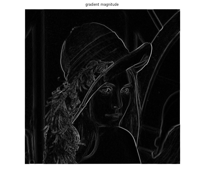
Differentiating Filters

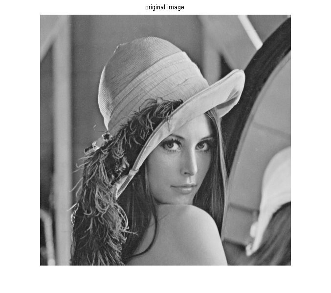
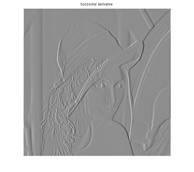
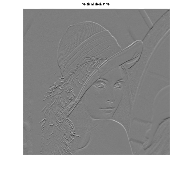
y = im2double(imread('image_lena512.png'));
figure(1), imshow(y),title('original image');

% compute gradient components (horizontal and vertical derivatives)
Gx=conv2(y , dx , 'same');
Gy=conv2(y , dy , 'same');

figure(3),imshow(Gx, []),title('horizontal derivative')
figure(4),imshow(Gy, []),title('vertical derivative')

% Gradient Norm
M=sqrt(Gx.^2 + Gy.^2);

figure(5),imshow(M,[]),title('gradient magnitude')

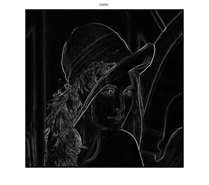
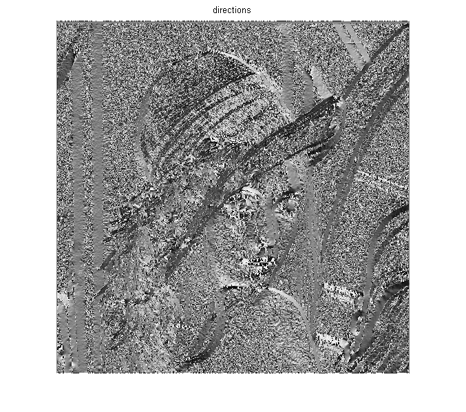
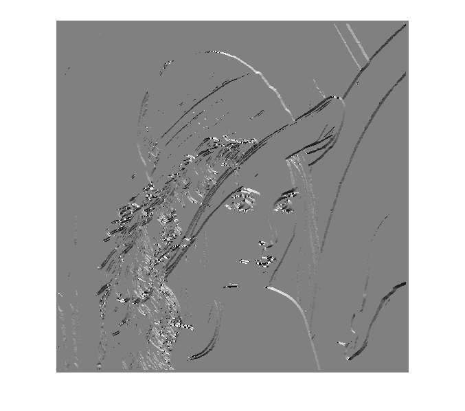
Compute image Principal Derivative (i.e. directional derivatives along axis)

% build the gradient image as a two plane image: the first plane contains horizontal derivatives, the second plane the
% vertical ones
Grad=zeros(size(y,1),size(y,2),2);
Grad(:,:,1)=Gx;
Grad(:,:,2)=Gy;

% compute Gradient norm
Norm_Grad = sqrt(Grad(: , : , 1) .^ 2 + Grad(: , : , 2) .^ 2);
BORDER = 3;

% remove boundaries as these are affected by zero padding
Norm_Grad(1 : BORDER, :) = 0;
Norm_Grad(end - BORDER : end, :) = 0;
Norm_Grad(:, 1 : BORDER) = 0;
Norm_Grad(:, end - BORDER : end) = 0;

% we change the sign of the derivative because the y axis is "increasing downwards", since in Matlab it correspodns to the row index
Dir_Grad=atand(- sign(Grad(:,:,1)).*Grad(:,:,2) ./(abs(Grad(:,:,1))+eps));

figure(2),imshow(Norm_Grad,[]),title('norm');
figure(3),imshow(Dir_Grad,[]),title('directions');

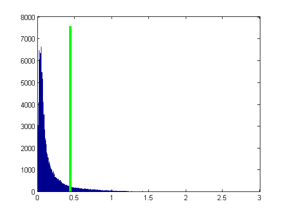
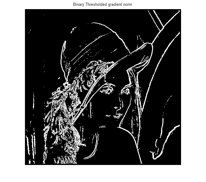
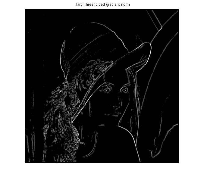
Hard Threshold - Play on the choice of the Threshold T

% Binary Threshold  - Play on the choice of the Threshold T
T = 5 * median(Norm_Grad(:));
% or choose the treshold using Otzu method (which is however meant for grayscale images, that are
% assumed to contain two classes of pixels, thus that their intensity follow a bi-modal histogram)
% [T , eff] = graythresh(Norm_Grad(:));

% arbitrary set the threshold
% T = quantile(Norm_Grad(:), 0.9); % 0.9 percentile

% compute the "gradient mask" by thresholding gradient magnitude
mask = Norm_Grad > T;

figure(4), imshow(mask), title('gradient mask')

% compute the histogram of gradient norm intensities
[hh , hh_bins] = hist(Norm_Grad(:) , 1000);

% show the histogram with the tresholded value
figure(7), bar(hh_bins , hh)
hold on
plot([T , T] , [min(hh) , max(hh)] , 'g' ,'LineWidth' , 3)
hold off

% perform Hard Tresholding using a mask
Norm_Grad_Binary = double(Norm_Grad > T);
Norm_Grad_Hard=Norm_Grad .* Norm_Grad_Binary;

% show Gradient Norm
figure(2),imshow(Norm_Grad,[]),title('Gradient norm');
% show the mask
figure(3),imshow(Norm_Grad_Binary,[]),title('Binary Thresholded gradient norm');
% show HT results
figure(4),imshow(Norm_Grad_Hard,[]),title(' Hard Thresholded gradient norm');
% show gradient directions in areas where gradient norm is large (i.e. over the gradient mask)
figure(5),imshow(Norm_Grad_Binary.*Dir_Grad,[])

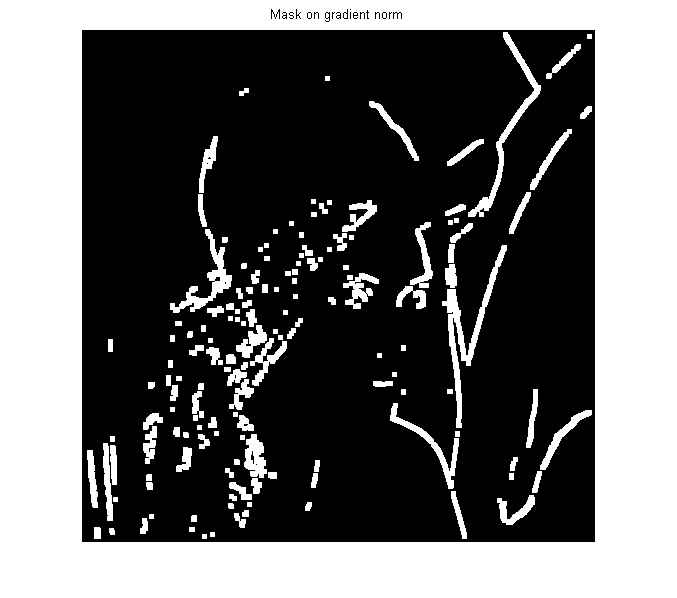
morphological operations on the mask

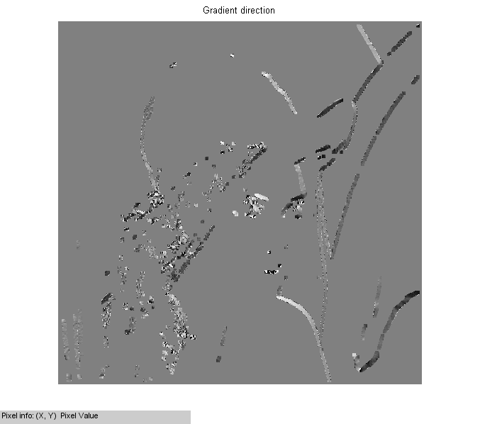
% dilate via convolution
% Norm_Grad_mask=double(conv2(Norm_Grad_Binary,ones(3),'same')>0);
Norm_Grad_mask = imerode(Norm_Grad_Binary , ones(3));
Norm_Grad_mask = imdilate(Norm_Grad_mask , ones(5));
figure(3),imshow(Norm_Grad_mask),title('Mask on gradient norm');

% show directions on the dilated mask
figure(4),imshow(Dir_Grad.*Norm_Grad_mask,[]),title('Gradient direction'),impixelinfo;

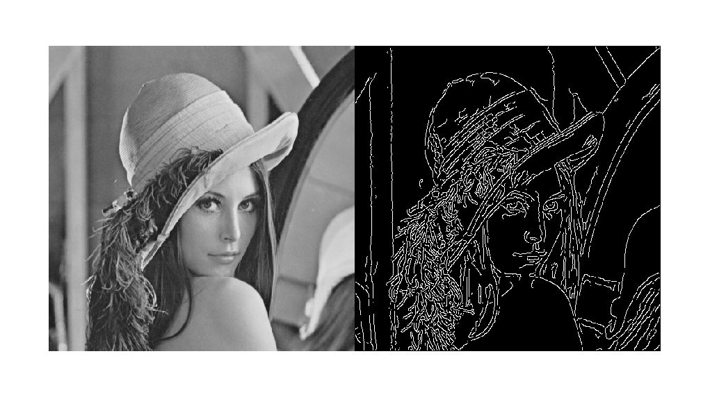
compute edges using Canny method (it includes nonmax suppression and histeresis thresholding)

edgs = edge(y, 'canny');
figure(6), imshow([y, edgs])

Published with MATLAB® 7.14