Contents

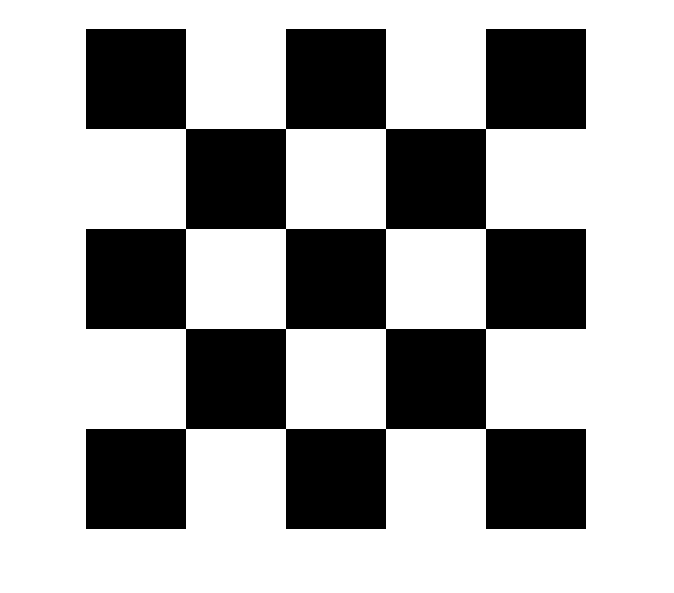
clear
close all
clc

% Goal: plot a few lines overlying this checkerboard

% load a checkerboard image
I = imread('checkerboard.png');

FNT_SZ = 28;

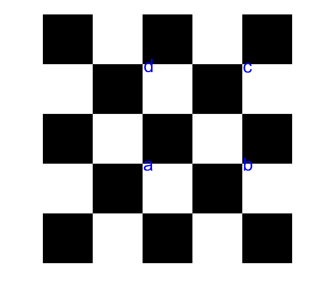
manually select points

figure(1), imshow(I);
hold on;
[x, y] = getpts();
% save points in the homogeneous cooridnate. It is enough to set to 1 the third component
a = [x(1); y(1); 1];
b = [x(2); y(2); 1];
c = [x(3); y(3); 1];
d = [x(4); y(4); 1];

draw the points over the image

text(a(1), a(2), 'a', 'FontSize', FNT_SZ, 'Color', 'b')
text(b(1), b(2), 'b', 'FontSize', FNT_SZ, 'Color', 'b')
text(c(1), c(2), 'c', 'FontSize', FNT_SZ, 'Color', 'b')
text(d(1), d(2), 'd', 'FontSize', FNT_SZ, 'Color', 'b')

compute the parameters of a few lines equation as the lines passing through 2 points

lab = cross(a, b); % this is the reference
lad = cross(a, d); % orthogonal to lab
lac = cross(a, c); % 45 degrees with lac
lcd = cross(c, d); % parallel to lab

check incidence relation

a' * lab % this should be zero when a \in lab
c' * lcd % indeed, this exactly corresponds to lcd(1)*c(1) + lcd(2)*c(2) + lcd(3)*c(3) = 0 that is the incidence relation

ans =
  -7.2760e-12
ans =
   3.6380e-12

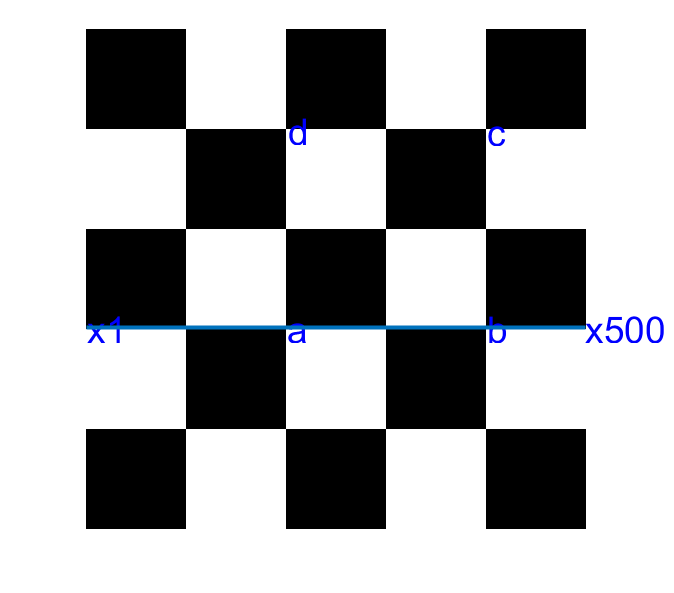
intersect these lines with the image borders

-> l: ax + by + c = 0; first column (c1) x = 1 -> a = 1, b = 0, c = -1 (remember that the first coordinate in matlab is the row, the second the column.

r1 = [0; 1; -1]; % parameters of top-most row
r500 = [0; 1; -500]; % parameters of bottom row
c1 = [1; 0; -1]; % parameters of left-most column
c500 = [1; 0; -500]; % parameters of right-most column

% compute the intersection between lab and the first column
x1 = cross(c1, lab); % point in homogeneous coordinates
x1 = x1/x1(3); % this normalization is required to plot the point over the Euclidean plan
                % bear in mind that x1 and \lamda x1 \forall \lambda ~= 0 are equivalent in P^2
                % to draw the point in the image plane, we need to take the point corresponding to x1 having third component
                % equal to 1
text(x1(1), x1(2), 'x1', 'FontSize', FNT_SZ, 'Color', 'b')

% do the same with the right most column
x500 = cross(c500, lab);
x500 = x500 / x500(3);
text(x500(1), x500(2), 'x500', 'FontSize', FNT_SZ, 'Color', 'b')
plot([x1(1), x500(1)],[x1(2), x500(2)], 'LineWidth', 3)

compute the angles on these images

computeEuclideanAngles(lab, lac) % 45 degrees
computeEuclideanAngles(lab, lcd) % parallel
computeEuclideanAngles(lab, lad) % orghogonal

ans =
   44.4242
ans =
  179.7135
ans =
   89.7106

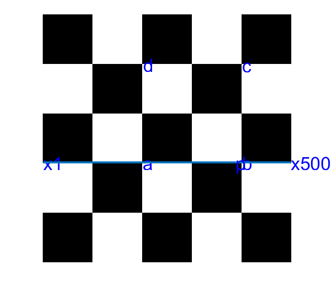
Verify the proporty any linear combination of a,b belongs to lab

lambda = rand(1);
mu = 1- lambda; % this is a convex combination. So points will be in between the two. The result holds for any combination

p = lambda * a + mu * b;
p' * lab

p = p/p(3);
text(p(1), p(2), 'p', 'FontSize', FNT_SZ, 'Color', 'b')

ans =
  -2.1828e-11

intersect parallel lines

vac = cross(lab, lcd)
vac = vac / vac(3) % look at this point, isn't it strange? It is a point at the infinity!
vab = cross(r1, r500)
vad = cross(c1, c500)

hold off

vac =
   1.0e+06 *
   -8.0002
   -0.0601
   -0.0002
vac =
   1.0e+04 *
    3.9802
    0.0299
    0.0001
vab =
  -499
     0
     0
vad =
     0
   499
     0

Published with MATLAB® R2017b